A deep critique of AI 2027’s bad timeline models

Disclaimers:

Thank you to Arepo and Eli Lifland for looking over this article for errors.

I am sorry that this article is so long. Every time I thought I was done with it I ran into more objections to the model, and I wanted to be as thorough as I could. I’m not going to blame anyone for skimming parts of this article.

Note that the majority of this article was written before Eli’s updated model was released (the site was updated june 8th). His new model improves on some of my objections, but I believe the majority still stand.

Introduction:

AI 2027 is an article written by the “AI futures team”. The primary piece is a short story penned by Scott Alexander, depicting a month by month scenario of a near-future where AI becomes superintelligent in 2027,proceeding to automate the entire economy in only a year or two and then either kills us all or does not kill us all, depending on government policies.

What makes AI 2027 different from other similar short stories is that it is presented as a forecast based on rigorous modelling and data analysis from forecasting experts. It is accompanied by five appendices of “detailed research supporting these predictions” and a codebase for simulations. They state that “hundreds” of people reviewed the text, including AI expert Yoshua Bengio, although some of these reviewers only saw bits of it.

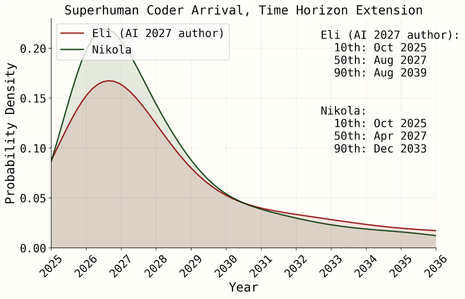
The scenario in the short story is not the median forecast for any AI futures author, and none of the AI2027 authors actually believe that 2027 is the median year for a singularity to happen. But the argument they make is that 2027 is a plausible year, and they back it up with images of sophisticated looking modelling like the following:

This combination of compelling short story and seemingly-rigorous research may have been the secret sauce that let the article to go viral and be treated as a serious project:To quote the authors themselves:

It’s been a crazy few weeks here at the AI Futures Project. Almost a million people visited our webpage; 166,000 watched our Dwarkesh interview. We were invited on something like a million podcasts. Team members gave talks at Harvard, the Federation of American Scientists, and OpenAI.

Now, I was originally happy to dismiss this work and just wait for their predictions to fail, but this thing just keeps spreading, including a youtube video with millions of views. So I decided to actually dig into the model and the code, and try to understand what the authors were saying and what evidence they were using to back it up.

The article is huge, so I focussed on one section alone: their “timelines forecast” code and accompanying methodology section. Not to mince words, I think it’s pretty bad. It’s not just that I disagree with their parameter estimates, it’s that I think the fundamental structure of their model is highly questionable and at times barely justified, there is very little empirical validation of the model, and there are parts of the code that the write-up of the model straight up misrepresents.

Unfortunately, in my effort to catalogue all the problems I found, this article has ended up being extremely long: it is now almost as long as the actual write-up I’m critiquing, with like a dozen fully original graphs to explain my issues. I have done my best to ensure there are no obvious errors, but I did this all in my spare time so I can’t guarantee perfection.

I have some familiarity with AI but I am certainly no expert. I am a computational physicist, so I do have familarity with computational modelling, and the actual model used in this forecast is fairly simple at only 300 lines of code or so (which is not necessarily a bad thing). In this article I will do my best to stay in my lane, and simply explain to you the assumptions and structure of their model, and then explain the various problems I have with what they did.

The authors of AI2027, to their credit, have been quite open to critique of their work, and have been generally helpful and kind when I corresponded with them about a few errors and critiques of their model. Eli Lifland, one of the authors of the model I’m critiquing, has kindly looked over this critique for factual errors. Although he disagrees with me on methodological and philosophical matters, he does agree with some of my critiques and has told me he will make several changes to the model write-up in response.

Even if at the end of this you think that I’m too harsh on the authors, I think this article still does a better job at explaining the AI 2027 timelines model than they do, so you can judge for yourself on it’s merit.

Remember that blogposts are error-ridden by default, and be appropriately skeptical of all of them, this one included. Please give the AI futures team an appropriate amount of time to respond as well. I will be crossposting this to the EA forum and lesswrong, so feel free to read the discussions there. If you see a clear-cut factual error in this or any of my other works, feel free to message me on substack about it. The somewhat messy code for producing my graphs can be found here.

Part 1: Time horizons extension model

Overview of their forecast

Note: This article is structured as a model explainer, going through each part at a time and critiquing them. It is not ordered by severity of problems, which vary between sections. I sum up my main issues in the conclusion.

There are many different parts to AI2027. This entire article is only about the “timelines” forecast, which is the first part of their chain of reasoning: an attempt to justify why we could get incredibly good AI coders in a very short amount of time.

The target of the forecast is the time until “superhuman coders”(SC), defined as an AI that can do the job of an AI researcher 30x as fast and 30x as cheaply as a human AI researcher. The methodology they used is described here, and the code is available here. The archive for the methodology at the time of writing is here, Eli has said he will be making several changes in response to this critique.

There are two methods modelled in AI2027, the “time horizon extension” method and the “benchmarks and gaps” method. There is also an “all things considered forecast”, which is a subjective adjustment to account geopolitics and macroeconomics. They present no further information about this “all things considered” forecast, so I will not discuss it.

In the first part of this article, I will focus on the time horizon extension method. I will return to their favoured benchmarks and gaps method afterwards. The main forecasters are Eli and Nikola, so I will be focussed on their parameters.

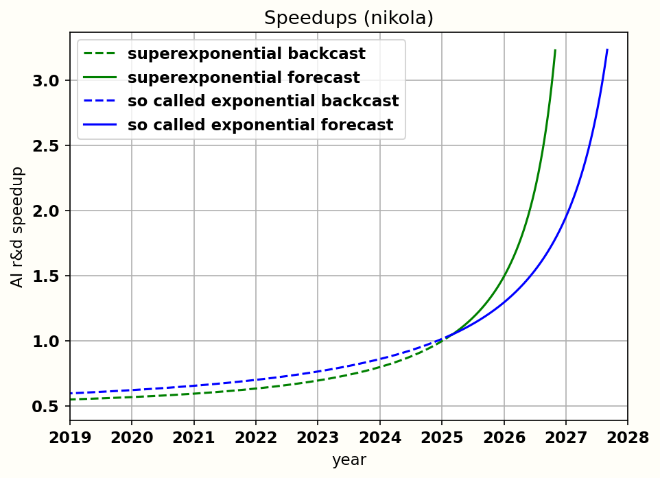
The time horizon method is based on 80% time horizons from this report, where the team at METR tried to compare the performance of AI on various AI R&D tasks and quantify how difficult they are by comparing to human researchers. An 80% “time horizon” of 1 hour would mean that an AI has an overall success rate of 80% on a variety of selected tasks that would take a human AI researcher 1 hour to complete, presumably taking much less time than the humans (although I couldn’t find this statement explicitly). The claim of the METR report is that the time horizon of tasks that AI can do has been increasing at an exponential rate. The following is one of the graphs showing this progress: note the logarithmic scale on the y-axis:

The METR report is quite recent and is currently not peer-reviewed and not replicated. The METR report seems like decent work to me, but it’s quite possible that there are subtle flaws that haven’t been outed yet, as happens fairly often in science. I would highly recommend checking out the report itself, which is pretty clear about it’s (understandable) limitations. For example the humans are not top experts and lack familiarity with the tasks they are doing: if we were comparing to top experts working on a familiar task the time horizons would be significantly lower. However, I will still be using this data as my primary comparison, as they have used it as a key part of their simulations.

In the simple time horizons model, each forecaster makes their judgement about what time horizon on METR’s benchmarks would correspond to a “superhuman coder”(SC), as defined above. Eli takes the limitations of METR into account in his forecast by placing the time horizon threshold for superhuman coders quite high (at 10 years). Nikola keeps it lower at 1.5 months.

The authors look at the METR data and their beliefs about AI and project a time horizon curve into the future, calculating when it meets the required time horizon for SC. They then add on a few months for the SC to get cheap, to get the total time required to reach SC.

After this, they do an “intermediate speedups” calculation to account for the speedup in development time as a result of AI progress, to get a new, much lower estimate for the time to SC (a lot more on this later).

There are a lot of parameters involved in this model. To account for uncertainty in those parameters, the value of each parameter is sampled from a lognormal distribution before running a simulation with those parameters: this is repeated many many times in order to give a range of likely values for the final results, like the uncertainty graph shown in the introduction. I don’t comment much on the lognormal sampling in this article, although this shouldn’t be taken as an endorsement.

Instead, I will be most looking at their point estimates in the middle of their distributions, which is where the peak of their lognormal sampling will be. These are their best guesses at the true value of parameter: a simulation with all their best guesses should look reasonable.

The “exponential” curve

So, let’s start with the assumptions going into method 1’s time horizon forecast, and one aspect in particular: the shape of the projection curve.

The authors divide their probability mass roughly equally between a “exponential” and a “superexponential” curve (each forecaster putting roughly 40% probability for each). I will cover the “exponential” curve first. My objections here are relatively minor, but will help set up the bigger problems later.

The exponential curve is fairly simple: you assume that the time horizon (H) doubles every T_0 months, where T_0 is the “doubling time”, an estimated parameter, from an initial value (H_0).The equation is

Where T is measured as time since the start of the simulation. The units used don’t matter as long as H and H_0 are both the same (I will use hours in the graphs) and T and T_0 are the same (I will use years).

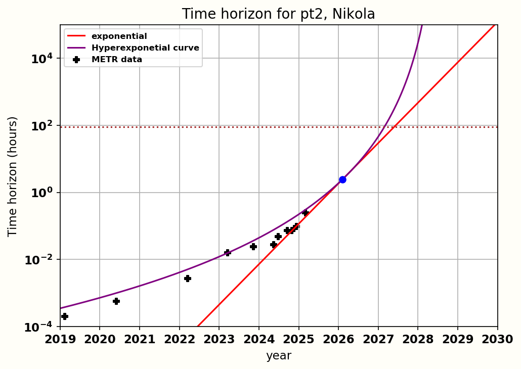
In the following graph, I show their median exponential curve in red, and the 80% CI bounds of their curve in dotted lines. I extracted the METR data from the graph in the previous section. The purple and blue dotted lines correspond to Nikola’s and Eli’s thresholds for superhuman coding, respectively.

Here we get to my first, small-ish problem with the forecast here. They estimate what the time horizon is now, and the doubling time is now, and this is taken as the input parameters for H_0 and T_0. They don’t include uncertainty in their estimate for H_0, setting it at exactly 15 minutes for every simulation with no uncertainty even though there are clear error bars on the METR graph above.

This is important, because as the METR report notes, it seems like horizon growth has been faster in the last year or so. But we don’t know whether or not this is the new normal or just noise or temporary bump where we’ll go back to the long term trend at some point. If you look at a graph of Moore’s law, for example, there are many points where growth is temporarily higher or lower than the long term trend. It’s the long term curve you are trying to estimate, you should be estimating the long term curve parameters, not the current day parameters¹.

One point I want to emphasize is that the “exponential” curve used here is not, as I first thought, the exponential curve predicted by METR, which is fitted to historical data. But you should hold your judgement on the fit for now, because this curve is not factoring in R&D speedups yet. I’ll go into it more later, but there's a reason I put “exponential” in quotes for the section title.

The “superexponential” curve

Okay, now let’s get into the much more problematic curve, the “superexponential curve”.

The first thing you should know is that “superexponential” is not the name of a particular curve, like a hyperbola or a sin curve or something. It just means “a curve growing faster than exponential”. There are infinite numbers of possible curves fitting this description.

So which one is it? Well, they don’t provide an actual equation (there are basically no equations provided in the entire timelines forecast). But they do provide a description:

“If the growth is superexponential, we make it so that each successive doubling takes 10% less time.”

So for example with their point estimates: we start in 2025 with an 80% time horizon of 15 minutes, with an initial doubling time of 4.5 months. Each subsequent doubling time is 10% shorter than the one before: so the second doubling time (to 30 minutes) is 4.1 months, the third (to an hour) is 3.7 months, etc.

Feel free to guess: What 80% time horizon does this predict for 2030?

BEGIN MATH

In this bit I will turn the description above into an actual equation for time horizon as a function of time.If high school math gives you bad flashbacks, feel free to skip this bit and trust me on this.

We will call the reduction rate alpha, which in this case is 10% or 0.1. That means the multiplicative factor which we will call r is 1-alpha or 0.9 in this case. Then each doubling time is given as T*r^n, where T is the initial doubling time n is the number of doublings.

So the total time is the sum of a geometric series:

The result of this sum is well known:

This is the equation they use in the github code. What they don’t do there is convert this into time horizon vs time, which is what I’ll be doing by rearranging the equation above:

And then combining it with the equation:

Once you deal with all the exponents and logarithms², and convert from r back to (1-alpha), you get:

Where H0 is your doubling time at t_start, alpha is your reduction fraction, T0 is the initial doubling time, and t is the time since the starting date of the simulation.³

In AI 2027, H0 is set at 15 minutes, Alpha is set at 0.1 (ie a 10% reduction in doubling time), and the initial doubling time is set at 4.5 months (with an 80% confidence interval of between 2.5 and 9). Using these parameters we get an equation of

Where t is in years.

END MATH

Okay, we can look at the actual curve now:

Just like before, the initial time horizon H0 parameter is not subject to uncertainty analysis. What’s much more crazy here is that the rate of doubling growth, which we’ll call alpha, wasn’t subject to uncertainty either! (Note that this has been updated in Eli’s newest version). As we’ll see, the value of this alpha parameter is one of the most impactful parameters in the whole model, so it’s crazy that they didn’t model any uncertainty on it, and just pick a seemingly arbitrary value of 10% without explaining why they did so.

So, now we can answer the question from before: what time horizon does the red curve above predict for 2030?

Well, if you plug it into wolfram alpha, you get a time horizon of “-2542 - 11372i”

Yes, that is negative, and that is an imaginary number in there.

What’s actually happening is that when the term in the brackets above hit zero, we end up dividing by zero, and hit infinity. Beyond that, we get a negative number to the power of a non-integer, which gives nonsensical complex numbered answers.

The infinity point for this equation happens at a time of t = To/alpha, and will always occur at some point, no matter what initial parameters you use.

In fact, this infinity point is completely independent of both the time horizon and the SC threshold. If you keep the same alpha and doubling time, you could start with a time horizon of a nanosecond, and have a superhuman coding threshold of 1 trillion years, and the curve will still claim that superhuman coding will arrive before the end of 2029.

And indeed, reddit user mambo-12345 tried modifying the simulation parameters to drop the initial time horizon to 15 nanoseconds instead of 15 minutes, and the resulting curve still had a peak for the estimated superhuman coder arrival at 2026.5 years and a median at 2035. Credit to them for inspiring me to take a closer look here:

Now I want to be clear: the fact that this equation always breaks after a certain length of time does not necessarily make it invalid or an incorrect choice. You could defend it by saying it’s merely an approximation over a short period of time, and indeed the AI2027 team model says that once a certain threshold of time horizon (shown as dotted lines on earlier images) is met, they switch to a different forecasting method.

But even with that defence… this is a weird curve, with some weird properties, and it would certainly not be the first curve that would come to mind if someone said the word “superexponential”. If I want to buy this model, I want to see some strong empirical or conceptual evidence that the curve makes sense in this context. In the rest of this article, I will show that no such evidence exists.

Conceptual reasons:

So, what arguments do they provide for superexponentiality? Let’s take a look, in no particular order:

Argument 1: public vs internal:

“The trend would likely further tilt toward superexponetiality if we took into account that the public vs. internal gap has seemed to decrease over time. It’s been rumored that GPT-4 was released 7 months after pre-training was complete, while it seems now there are much smaller delays; for example according to the announcement video Grok 3 was released a month after pre-training was complete.”

Now, this is already a bit of a sketchy point. The METR data was tested on the models at their external release date, not the models at their internal release date. This argument seems to assume that they would do just as well, but probably GPT-4 did improve on benchmarks during that 7 months after pre-training.

But even if we do accept this argument, this effect points to a slower growth rate, not a faster one. If earlier models had a longer time between development and deployment than newer one, that means that the actual gap between model improvements is in reality longer than it looks on graphs.

Suppose we say the pretraining to training gap used to be around 7 months for each model, but decreased linearly between GPT4’s release around 2024 from 7 months to 1 month now (probably not accurate, but I’m just demonstrating a point). If we adjust the data to show the actual internal release of the model we would get the blue curve below:

Not only does the blue curve have a slower doubling time at the present, it also makes the data overall less concave (at least for this toy example). This shows that the apparent recent speedup in double time could be partly an illusory artifact of people releasing models earlier. Take caution here, as the effect on the concavity will depend in complex ways on the actual relative values of the internal gaps (a fully linear decrease will not affect the concavity at all, only the slope). The general rule of thumb is that the slope will look steeper than it actually is if the internal deployment gap is decreasing, and vice versa, and since the time period of decreasing gaps being discussed is very recent, it would, if valid, most likely offset the recent apparent speedup, at least slightly.

Now don’t take the blue graph too seriously, I don’t know the actual internal deployment gap beyond the ones stated here, and as I mentioned we can’t assume each model had the same time horizon at internal release as it did in external release. Regardless, my point is that either the argument above is invalid, or it points in the opposite direction to what the authors are arguing for. Eli has agreed to remove this argument from the document.

Argument 2: difficulty gap:

“Conceptual: It seems like for humans the gap in difficulty between 1 month and 2 month tasks is lower than between 1 day and 2 days. It’s unclear whether this will transfer to AIs though, given that thus far relative to humans they have solved tasks more strongly with knowledge than with general reasoning. Perhaps this could be the case if extending to each successive time horizon requires doing large amounts of training on tasks of that horizon.”

The phrase “gap in difficulty” is a little ill-defined here, but from context I assume they mean something like how much extra skill is needed. Now, remember, the curve says each successive doubling makes the gap 10% easier. So the actual claim they are making is that the difficulty jump from 1 to 2 months is 60% easier than the jump from 1 to 2 days.

“Going from 1 week to 1 year might be ~2x easier than going from 1 hour to 1 week. 1 week tasks can be much more complex than 1 hour tasks, but we project there aren’t as many extra skills needed to go from 1 week to 1 year.”

This similar justification is hidden away inside a graph in a different part of AI2027. The math actually checks out for this one, there are roughly 6 doublings in each gap, and 0.9^6 is around 0.5.

I’m skeptical that these statements are true for humans, and I’m extremely skeptical that this is true for LLM’s for a similar reason: there are much more available examples and tutorials for shorter tasks than for longer ones. I feel like a 1 week job can be done by an amateur following tutorials and copy pasting code, whereas a 1 year job is something that requires someone with years of experience to do well. Given that LLM’s today rely on massive amounts of training data, it seems like this would be an even bigger deal for them.

I don’t have experience in AI R&D labs, so don’t take my word on this one, but the argument seems weak and underdeveloped. If I were them I would seek out an actual metric here to judge the “2x easier” claims, and actually demonstrate that it follows this “each doubling is 10% easier” claim.

Argument 3: recent progress:

“The METR report finds a 3.5 month doubling time for 2024-2025, compared to a 7 month doubling time for 2019-2025. This is based on few data points. Scaling up agency training provides a potential reason for the trend, as discussed in Section 7.2.2 of the report.”

A recent speedup is quite weak evidence for this specific type of super exponential curve. As I will show later, you can come up with lots of different superexponential equations, you have to argue for your specific one.

That leaves the “scaling up agency training”. The METR report does say that this might be a cause for the recent speedup, but it doesn’t say anything about “scaling up agency training” being a superexponential factor. If agency training only started recently, could instead be evidence that the recent advances have just bumped us into a faster exponential regime. Or, as the METR report notes, it could just be a blip as a result of recent advances: “But 2024–2025 agency training could also be a one-time boost from picking low-hanging fruit, in which case horizon growth will slow once these gains are exhausted”.

Argument 4: infinite time horizons:

“Another argument for eventually getting superexponentiality is that it seems like superhuman AGIs should have infinite time horizons. However, under the definition of time horizon adapted from the METR report above, it’s not clear if infinite time horizons will ever be reached. This is because AIs are graded on their absolute task success rate, not whether they have a higher success rate than humans. As long as there’s a decreasing trend in ability to accomplish tasks as the time horizon gets longer, the time horizon won’t be infinite. This is something that has been observed with human baseliners (see Figure 16 here). Even if infinite horizons are never reached, the time horizons might get extremely large which would still lend some support to superexponentiality. Even so, it’s unclear how much evidence this is for superexponentiality in the regime we are forecasting in.”

This is the only argument that actually argues that the curve should be infinite in nature, and it’s an argument the authors aren’t willing to endorse.

I don’t buy this claim. Just think about what a time horizon of a thousand years means: this is a task that would take an immortal CS graduate a thousand years to accomplish, with full internet access and the only requirement being that they can’t be assisted another person or an LLM. An AI that could accomplish this type of task with 80% accuracy would be a superintelligence. And an infinite time horizon, interpreted literally, would be a task that a human could only accomplish if given an infinite amount of time. I think given a Graham’s number of years a human could accomplish a lot, so I don’t think the idea that time horizons should shoot to infinity is reasonable.

And… that’s it. That’s basically all the justification given in the report. The shape of these curves are one of the most crucial factors determining the final topline result, the choice of curve is extremely weird, and yet most of these arguments have nothing to do with why we should prefer this specific curve over any others.

Intermediate speedups

Now if you read the justifications in the section above, you might be a little confused as to why they didn’t raise the most obvious justification for superexponentiality: the justification that as AI gets better, people will be able to use the AI for r&d research, thus leading to a feedback loop of faster AI development.

The reason for this that they explicitly assume this is true and apply it to every model, including the “exponential” and “subexponential” ones. The “exponential” model is, in fact, also superexponential in their model.

(Note: in Eli’s newest model the speedup model is way more complicated, I will touch on this later)

In the code they use an equation (with sparse justification) for how the algorithmic speed of research will be sped up compared to 2024:

Where V is the rate of AI speedup, m_0 is the speedup rate at simulation start m_f is the speedup rate when superhuman coders are reached, p is amount of AI progress made since simulation start⁴, in terms of “2024 months”⁵, and p_f is the length of time required to reach SC without any intermediate speedups.⁶

Note that obviously, progress on AI did not start in 2025, and 2025 is not a special term in time. The V’s in this forecast are all relative to each other: you can calculate V’s in the past by setting the progress p as a negative number.

Then they average this with V_compute, which is just set as exactly one because compute is not affected by algorithmic progress:

The actual code consists of jumping forward in time by a timestep of dt (one day), and calculating how much progress in 2024 months is made in that timestep, until the total progress reaches p_f:

You can actually create an analytical equation out of this, by rearranging and integrating this, but it’s a giant pain and not robust to changes in simulation parameters. Instead, they do the simulation until their progress p hits p_f, and that’s the time to SC.

This might be a little confusing, so I’ll step through an example. At a progress time of zero, the value of V is 1.1 (in median simulation). this means that when one day in real time has happened, slightly more than one days worth of AI progress has occurred on the AI timeline. Then the next day, the progress is now 1.1 day, so V_total, the speed of AI development, is now just a little bit higher, meaning that one day is now worth slightly more than 1.1 days of AI progress, so the total amount of progress is now slightly more than 2.2 days. This continues and compounds, until the AI progress hits the predicted length till SC from earlier.

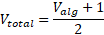
The fun thing about this is that we can continue the curve back in time simply by setting the timestep to be negative, to get a backcast instead of a frontcast. After all, the unit we are using is “2024 months”, which is valid back in time as well as forward. To be clear, they don’t do this, I’m the one doing this in order to see how valid their curves are.⁷

So here is a graph of the total velocity vs time, with the backcast in dots, for Nikola’s curve and their point estimates for H_sc, T_0, etc :

So a backast towards 2022 predicts an AI R&D speedup factor of around 0.6 for both type of forecasts. With a current factor of about 1.1, this means that a backcast is modelling that current AI progress is 66% faster than it was in 2022.

This does not match with Nikola’s own statement in the appendix:

“Nikola’s current guess is that algorithmic progress is 3-30% faster with AI chatbots and copilots from the 2022-2024 period than it would be if AI researchers didn’t use them.”

I think I know what went wrong here, actually. See, in the code they actually do include the 3-30% estimate. They do this by setting the present day velocity value m_0 (present_prog_multiplier in the code) to be above one, in line with the “3-30% better” estimate (median value being about 1.1). They thought that by setting the present day R&D factor to 1.1, they would ensure their model fit their estimate by default.

Problem is, that multiplier value of 1.1 is a meaningless number on it’s own. What matters is the relative speed factor. They didn’t realise that the equation implies that the R&D factor a few years ago could be less than 1. If you actually want to make the model work, you’d have to ensure that the present day R&D factor was 1.1 and also that the R&D factor in 2022 was 1. To get that working with the current equation, you’d have to set the final R&D factor at SC level to… 1.17, aka barely any speedups at all. The easier explanation is that the totally unjustified algorithmic velocity equation they used is bad.

Finally, I’ll show you my attempt at producing the actual, final curves for each model. First, we can get the conversion rate between actual months and 2024 months:

This is an equation for progress in “2024 months” as a function of real time. The equations I showed in the exponential and superexponential sections of this article show time horizons as a function of “2024 months”. So we can substitute between the two to get a final graph of time horizons as a function of real time:

This is just Nikolas curves, Eli’s aren’t that different. We can see that the median “superexponential curve” has been doubly squished, and doesn’t match with the historical data at all. The “exponential curve” is actually superexponential, and while closer to the data it’s not a particularly strong fit. I assume the real data would mostly be within the 80% CI of these curves, but I don’t think the actual data should be an edge case of your model.

So, to finish off the “superexponential” the particular curve in their model does not match empirically with data, and as I argued earlier, it has very little conceptual justification either. I do not see the justification for assigning this curve 40% of the probability space.

Have AI 2027 been sending out a false graph?

In one of the sidenotes in the AI 2027 short story, entitled “why we forecast a superhuman coder in early 2027”, the authors present the following graph:

Versions of this graph have been subsequently shared on AstralCodexTen and Daniel Kokotajlo’s (another AI futures author) twitter. Scott alexander referred to it as “AI 2027's prediction”, and Daniel as showing that (although way too early too call), that a new LLM datapoint “was consistent with AI 2027's controversial superexponential prediction”

Now, I feel a little bad about writing this section, because I’ve been badgering various members of AI futures team about this curve for a few weeks now, and they have fixed a few of my initial issues with the image, like when Scott Alexander posted a 50% time horizon graph that was mistakenly mislabelled as an 80% time horizon graph (I pointed this out and he fixed it).

This initial curve above, still on the AI2027 website⁸, has two issues that were fixed in subsequent versions:

First, the last datapoint, claude 3.7 sonnet, is incorrect. It should be 15 minutes, not 30. This is fixed in subsequent versions, but remains on the actual website itself.

Second, two datapoints are missing from the graph that were present in METR data: the two earliest ones, GPT2 and GPT3. When I asked them about this, they stated that they removed them because their time horizons were too low to be meaningful, but are you really going to say that 2 seconds (GPT-3) isn’t meaningful, but 8 seconds (GPT-3.5) is? It’s extra questionable to do this because putting in those datapoints makes the curve look worse, which you can see in the most recent version of the image (note that this is the 50% horizon, not the 80%):

Even with this graph though, I still have problems , the caption says that “each doubling gets 15% easier”. Except that in all of their modelling, it doesn’t get 15% easier, it only gets 10% easier. As we saw earlier, this parameter is extremely important, so it’s concerning that they don’t have their data straight.

Next: This curve is not the curve from the AI2027 forecast. Eli has confirmed to me that this is not produced by the timelines curve, it is merely “meant to give a rough sense” of their model, and “not be super precise”. Some differences with the model:

First point: they don’t state which model is being used, the time horizons or the benchmarks and gaps. It can’t be the superexponential curve without speedups, because you can clearly look at times between doubling and note that they do not, in fact, decrease by a constant amount in time. (In the original 80% timeline curve, 8 secs to 16 secs is roughly 1.5 years, 16 sec to 30 sec is only 1 year, which is way more than a 15% drop). So maybe it’s the superexponential curve with speedups? But in that case, which superexponential curve? The shape of this curve depends on a number of different parameters, none of which are supplied, and it differs between the two different forecasters. Why isn’t this labelled “eli’s” curve, or “nikolas” curve, and why aren’t any parameters given? Also, all the timeline forecast modelling is for 80% timeline curves. The timelines forecast does not do any projection of the 50% curve like is done here. Also, they adjusted the curve when they added datapoints: this is not done in their simulations. You can also check the code, there is no trace of this graph there.

What is the point of a graph like this, if it’s not the curve from any version of their actual model? If you compare with the actual median curves in the previous section, neither the exponential nor superexponential curve matches with this “rough sense” model. People will look at this curve and make judgements about whether the fit looks good, whether recent data fits the curve, etc, and then assume that means that it provides evidence about the quality of the AI2027 prediction. This is simply not the case.

I am concerned that Scott and Daniel have graphed new LLM performance on this unrelated curve and presented it as evidence in favour of their model, even if they have been clear that it is “weak” evidence. It’s wrong to present this curve as “AI 2027’s prediction”, as Scott did.

In response to my critique, Eli whipped up some code to check the graph against actual runs from his simulations. He generated the following graph of actual simulations, selecting only the ones that reach SC in march 2027 (ie, matching the AI 2027 short story), compared to the graph above (in purple “reference timeline”). He now agrees that the graph is not representative of the model. I encourage him to explore these graphs more: remember I am only graphing the median parameters in this article for convenience, so something like this could be quite useful for elucidating more about what is happening in the actual model.

Some skepticism about projection

I want to inject some wider skepticism about this project of projection. Here are two curves, fitted to the METR data:

The difference in fit between each curve is negligible. Certainly they both fit better than the curves actually used in AI 2027.

One of these curves is a fitted version of the “superexponential” curve from earlier, without intermediate speedups:

Parameters are H0 = 9.5 minutes, T0 = 0.3855 years, Alpha = 8.38 %

The other curve is a one I am introducing here, and calling “quadexp”.

Where A and B are fitting parameters, H0 is the time horizon at t =0, and t is the time since simulation startpoint. Parameters are H0 = 9.5 minutes, A=0.1,B=2.17.

Now, let’s zoom out and see what each curve predicts for the future:

Both curves have 3 fit parameters, both are “superexponential”, both appear to fit the data very closely. But the green graph predicts a literally infinite time horizon by 2030, whereas the blue graph predicts a time horizon of a few months.

And of course… neither are the actual curve used in the AI 2027 forecast. In an earlier draft I went to the trouble of actually solving the equation for a simplified version of the superexponential curve with intermediate speedups, with no extra gaps and assuming V_total =V_algorithmic. After a lot of integrations and substitutions, the full equation would be something like:⁹

With six parameters of H0, alpha, m0, mf, Hsc, and T0. The full equation is even more complicated, and would also include the cost and speed gap, the internal delay amount, and V_compute, for a new total of 9 parameters. Method 2 which we’ll get to later adds a further 5 or so parameters, and Eli’s newest method adds even more.

I suppose you could argue that in the real world, all those parameters do affect the rate of AI progress, so isn’t it good modelling to put them all in?

But there are also way more factors that aren’t accounted for, like the amount of available data, economic growth, AI regulations, total investment, the degree of AI uptake among the public, the amount and distribution of talented people at AI companies, etc. And you don’t just need to try and predict what these values will be, you also need to predict how all these parameters will interact in such a way as to finally affect the rate of compute progress. To untangle this web, you need a degree of precision, empirical evidence, and conceptual rigour that the authors of AI 2027 do not meet.

I agree with the authors of METR report when they decide against fitting their data to anything above a regular exponential¹⁰. There are only 11 datapoints, having a model with 6 parameters (or 9, or 14, or more) is just too much. As we saw above, with this few data fitting even three parameters can lead to wildly different results. More complicated does not equal better.

Which brings us to the next model:

Part 2: Benchmarks and gaps and beyond

The benchmark part of “benchmark and gaps”:

When some of the issues with the time horizons forecast were pointed out, the AI 2027 authors have defended themselves by pointing out they actually did two models, and the time horizon model that we have discussed so far is a simplified one that they do not prefer. When you use their preferred model, the “benchmark + gaps” model, the assumptions of the time horizon model are not as important.

I disagree with this defence. In fact, I think that method 2 is in many ways a worse model than method 1 is. I think in general, a more complicated model has to justify it’s complications, and if it doesn’t you end up in severe danger of accidentally overfitting your results or smuggling in the answer you want. I do not believe that model 2 justifies its complications.

Method 2 starts by predicting how long it would take to achieve a particular score (referred to as “saturation”) on Re-bench, a benchmark of AI skill on a group of ML research engineering tasks, also prepared by METR. After that, the time horizon extension model is used as with method 1, except that it starts later (when Re-bench saturates), and that it stops earlier (when a certain convoluted threshold is reached). After that stopping point, 5 new gaps are estimated, which are just constants (as always, sampled from lognormal), and then the whole thing is run through an intermediate speedup model. So any critiques of model 1 will also apply to model 2, there will just be some dilution with all the constant gap estimates and the “re-bench” section.

So, let’s start with the re-bench “saturation”. They are forecasting how long it will take to get to a re-bench score of 1.5, which they estimate to be the performance of “the best human” on the task suite inside the re-bench benchmark. To find this, they “extrapolate” the data by “fitting” a logistic curve, shown below:

The reason I have put “fitting” and “extrapolate” in quotes above is that it is basically useless to actually try and extrapolate a logistic curve. Here is what happens when I extracted their data and ran a fitting algorithm to a simple logistic curve:

That’s right, the fit predicts that re-bench is already nearly at it’s maximum value. I wouldn’t say this is true (although I would find it pretty funny). The actual truth is that precisely predicting where a logistic curve will saturate from the data alone is for the most part impossible until you’ve already clearly passed the inflection point. We could pretend that the rightmost point is evidence that RE-bench has already started saturating, but I don’t think there is enough evidence to say that from the data alone.

So what do they do instead? They just guess the upper limit, and only fit the remaining parameters. They declare, with basically no evidence, that the LLM score on Re-bench will reach an upper limit score of 2.0, 33% better than their estimate for the best performance by a human expert.

They then declare that “Changing the upper bound doesn’t change the forecast much”, because they tried upper limits between 1.75 and 2.25 and it didn’t affect the results substantially. But of course it didn’t, because both of these bounds are still substantially above best human performance! If they’d changed the upper limit to be 1.4 instead, the code would predict re-bench saturation taking a literally infinite amount of time.

I could go on further, but it doesn’t actually matter. See, step 1 of method 2 is to do this RE-bench saturation calculation.

Step 2 is to throw this calculation in the trash.

I’m serious here. Look at the code. The variable t_sat_ci, the “CI for date when capability saturates”, is set by the forecaster, not calculated. There is no function related to the RE-bench data at all in the code. Feel free to look! It’s not in the updated code either.

If you want further proof, take a look at the distribution of dates to meet their saturation threshold that is presented in their appendix as the result of the logistic RE-bench fitting:

And compare it to their sub-graph “time to saturation”, which is hidden in the big graph graphing like 20 different parameters:

I’ve checked, and these absolutely are meant to be the same parameter. They do not match at all. And we can again look at the code: The 80% CI given by each forecaster is different to each other, and neither correspond to the distribution of the phantom RE-bench calculation. Eli gives an 80% CI of saturation between september 2025 to january 2031, and Nikola gives an 80% CI of saturation between august 2025 and november 2026. Neither of these are the same as the 80% CI in the first of the two graphs, which is early 2026 to early 2027. Both distributions peak like half a year earlier than the actual Re-bench calculation, although Eli’s median value is substantially later.

No part of their RE-bench “logistic curve fitting” actually makes it into the final simulations, even though it’s half the name of the “benchmarks and gap” method. Eli has told me that the final estimates for saturation time are “informed” by the logistic curve fitting, but if you look above they are very different estimates. Nikola’s peak is in mid to late 2025, which is way outside of their 80% confidence interval for the RE-bench scores. The empirical RE-bench data seems to be a very tiny part of their reasoning here, misleadingly presented as if it was a major part of their simulation.

This is probably the most clear-cut falsehood in the appendix, because they really don’t mention this, and leave out the “time to saturation” parameter entirely, even though you can clearly see it in the sub-graph hidden among all the other parameters. This absolutely should have been made clear: Eli has stated he will fix this in a website update.

The time horizon part of the model

Okay, so we’ve just thrown out the re-bench part of the appendix. What happens next? Well, next, we do another time horizons calculation, using basically the same methodology as in method 1. Except we are starting later now, so:

They guess the year that we hit re-bench saturation.

They guess the time horizon at the point we hit re-bench saturation.

They guess the doubling time at the point when we hit re-bench saturation.

They guess the velocity of R&D speedup at the point when we hit re-bench saturation.

Then, they use these parameters to do the time horizons calculation from part 1, with a lower cut-off threshold I will discuss in a minute.

And they don’t have a good basis for these guesses, either.I can see how saturating RE-bench could you give you some information about the time horizon, but not things like the doubling time, which is one of the most crucial parameters that is inextricably tied to long term trends.

And the estimation of doubling time is weird. The median estimate for doubling time at re-bench saturation is around 3 months, which is 33% lower than their current estimate for doubling time. Why do they lower it? Well, partly because under the superexponential model there would have been speedups during the re-bench saturation period. But this speedup due to superexponentially is applied to every model, including the exponential and subexponential ones! The whole definition of an exponential model is that the doubling time isn’t changing, but if you pick it in this model you effectively end up with a model where doubling is superexponential for an arbitrary period beforehand, then stops and becomes exponential instead.

What was the point of the re-bench time estimation? What does this add to anything? You are trying to guess the time until we hit a time horizon threshold, but we have just started the simulation later and just guessed what all the parameters will be like at an arbitrary point. This whole procedure seems completely unnecessary. The entire time horizons section is based around the METR data today, so they should start today. There is really no point in having the re-bench section at all.

The other main difference is that this time horizons model only goes to a lower threshold, corresponding to when AI hits the following requirement:

“Ability to develop a wide variety of software projects involved in the AI R&D process which involve modifying a maximum of 10,000 lines of code across files totaling up to 20,000 lines. Clear instructions, unit tests, and other forms of ground-truth feedback are provided. Do this for tasks that take humans about 1 month (as controlled by the “initial time horizon” parameter) with 80% reliability, add the same cost and speed as humans.”

Despite differing by 2 orders of magnitude on the time horizon required for SC in the first method, when it comes to meeting this benchmark they are both in exact agreement for this threshold, which they both put as a median of half a month. This is weird to me, but I won’t dwell on it.

I will show the graphs here for the exponential and superexponential time horizon curves predicted by Eli and nikola. I’m taking the geometric mean of their estimates in the code for this (as it was sampled lognormally). I will show the new threshold for stopping the simulation (about a 100 hours) as a brown dotted line. In Nikola’s curve, the median time to saturation is about 1 year:

This barely changes the superexponential curve from the one in the time horizon case, but the exponential now has a much steeper slope.

Next, for eli, the median time to saturation is about 1.8 years, but the rest of the parameters are nearly the same as for nikola:

The superexp is sorta in the right ballpark, but the exponential is nowhere near the data. It’s like this simulation predicts AI progress to freeze in place for two years, then suddenly start again and continue exactly the way it was before.

One effect of this is that there is no longer a large difference between the superexponential and exponential curve, because the gap between the starting time horizon and the cut-off threshold is no longer that large. Of course part of the reason for that is the assumption that doubling time has sped up even in the exponential case, which I earlier argued doesn’t make a ton of sense.

As a result, changes in the superexponential probability parameter doesn’t have a large effect on this model, although it will have some effect if the lognormal sampling picks a high threshold or low time horizon.

Now remember, this is the curve before speedup adjustments. However I have decided not to invest the effort into graphing the actual curves for this model due to the extra complications involved. Given the big differences between them, most of these curves will not match the historical data.

The gap model

I don’t have as much of a critique for this last bit of the model, because it’s fairly simple. In this model, the time horizon estimation is somewhat less important, because once the model has reached the lowered threshold described above, it switches to modelling a series of “extra gap” that need to be crossed, one after another, as they show in the diagram:

Note that this is not proportional. Using their point estimates, they have roughly 18 months for the time horizon step, and then (3+6+1.4+1.7+6.9+5.5= 24.5 months for the other steps.¹¹ So the time horizon step is still highly important to the results. Really, any part of it could be important to the results, if it turned out to be the main bottleneck in the simulation.

These gaps are just direct estimates from the authors, sampled lognormally. I think commenting too much on these gaps would be out of my lane, but I will highlight a problem with the “engineering complexity” gap. In this gap, they state that the lines of code (LOC) will depend on the time horizon, which they assume has a doubling time of “3 months” at this point in the simulation:

However, they are already explicitly modelling the doubling time in their simulation. And their median estimate for the doubling time at Re-bench saturation is already 3 months, when their estimated time horizon is only 2.5 hours. They would have had to go a further 8 doublings to get to this point in this simulation, which in the superexponential case would have reduced the doubling time further to only 1.2 months. So for this gap, at least, their guesses are inconsistent with the rest of their simulations.

I think my main problem with the gaps is that they correspond to guessing things about a future technology that doesn’t exist yet, so there's no good way to validate them. But I want to stay in my lane here, you can decide for yourself if they are reasonable guesses.

To finish up, I will show that in this original version of model2, the intermediate speedups have a large effect on the results, by showing Eli’s simulation with and without R&D speedups:

One thing I want to stress is to not be fooled by the peak being in the same place into thinking these simulations give the same answer. I suspect these peaks are due to the gaps, not the time horizon. If you look at the actual median SC estimate, it’s 4 years longer without the speedups.

What about Eli’s recent update?

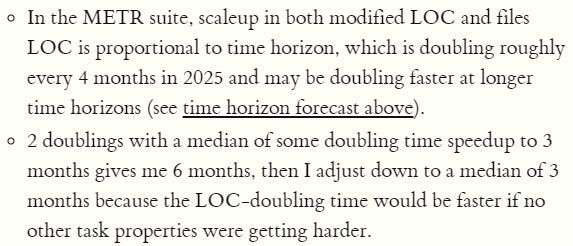
I’d already written this critique when the site updated to show that one of the authors, Eli lifland, has released a new model, with timelines that are generally a year or two later than the original model. (although it is called the may 2025 update, they only went public with it on the website in june). This new model pushes Eli’s estimates of SC arrival back by about two years for both models, and adds a number of complications to the model. In his favoured model 2, the median arrival time for SC is now 2030. I will go over a few initial thoughts about the new model but ultimately I will not pass proper judgement until Eli writes up more about the model.

The first clear improvement is that he included uncertainty in the superexponential reduction fraction alpha.

The second is that he showed quite a few experiments on the effects of different assumptions on the model such as R&D speedups and superexponentiality, which are worth checking out.

However most of my objections above are unchanged. The “re-bench” step still has no reason to exist, there is no extra conceptual justification for anything, there is still no validation with empirical data, etc.

And one change I think makes no sense is the treatment of superexponential curves:

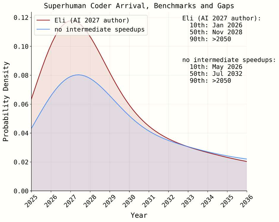
See, now instead of a 40% chance of a superexp curve, the code now claims there is a ~90% chance of having a superexp curve eventually, it’s just that sometimes it starts off delayed. Now they define a series of time horizons and the probability of hitting superexponentiality at that point:

They pick a random number, and then pick the leftmost dot that is greater than this number, and assume that from this point superexponentiality starts. So if you roll a 0.5 as your random number, the largest time horizon lower than this is 0.045 months, so that’s when the superexponentiality starts.

So for example, using the threshold of 0.045 months, which has roughly a 15% chance of being picked, the curve looks like this:

There’s a 25% chance that the superexp is the same as in the initial model, a 10% chance of subexponentiality, and the remainder of the probability will look like the graph above, just starting at a different point.

I… don’t get it. Why assume that the curves look like this? This is explicitly not due to speedups from AI R&D, and you can no longer justify it by gesturing at the seeming uptick in recent METR data, because your model says we are still exponential at that point. Even if the “internal gaps are decreasing” argument wasn’t nonsense, you also wouldn’t be able to apply that either. The only justification left is the argument about progress from 1 week to a year being easier than progress from 1 hour to a week, but that wouldn’t justify this weird delayed superexponential. I hope that Eli will justify this when he writes up the model.

Now, the other main change is that Eli has made the “intermediate speedups” model way, way more complicated, adding in labor pools, research stock. The original algorithmic speedup equation is still in there, but now it’s fed through a series of equations for labor pool, speedups, compute, etc. The ultimate effect of these does seem to have resulted in longer timelines estimates than in the original model.

The majority of these new equations or parameters are not listed, explained or justified in the additions to the appendix at time of writing, and the fit of this new model to historical data is not attempted. Because of this, I do not have the time or motivation to dig into them. I will repeat my earlier argument: a more complicated model is often a worse model, especially with sparse and noisy data.

I believe Eli is still in the process of writing up this new model in more detail, so I will refrain from commenting further until then. Besides, this is not the model that went viral anyway, and it predicts years longer timescales than the AI2027 short story.

Six stories that fit the data

To finish up, I want to make a general point about the inherent difficulty of a forecast like this. In the following graph I have shown six curves, each showing a different model of the future.

I want to emphasise that I do not think each curve is equally likely. In fact, I endorse none of them. I am simply showing a number of ways you could build a model in the vein of AI2027, pushing different arguments about AI timelines.

The Green hyperexponential curve comes from someone who decides that the original “superexponential” curve is correct, but that the speedups will be 20%, not 10%, and that the 2024-2025 rate of growth is valid. They dismiss the lack of fit with the early datapoints because they were too small to be valid. This model predicts that we’ll hit both Nikola’s and Eli’s SC benchmark in mid 2026.

The golden curve is the method 1 superexponential curve (including speedups) from AI 2027 using all of Nikola’s median parameters. This predicts hitting Nikola’s SC benchmark in mid 2026 and Eli’s SC benchmark at the end of 2026.

The red, “new normal ” curve thinks that AI will progress exponentially, but that the recent 2024-2025 period is the new normal, and that time horizons will continue with this new, faster doubling time for the foreseeable future. They ignore all earlier datapoints, claiming that they were following an earlier, slower trendline before the advent of something (like agency or chain of thought) kicked off faster progress..This predicts hitting Nikola’s SC benchmark in mid 2027 and Eli’s SC benchmark at mid 2029.

The blue, “quadexp” curve is the one from the “tale of two data fits” sections. In this narrative, progress is slowly speeding up, and to find out how quickly we take the simplest 3 parameter model that works with all the historical data and just draw it out. This predicts hitting Nikola’s SC benchmark in mid 2029 and Eli’s SC benchmark at mid 2031.

The purple curve is the one proposed by METR. They see that historically, time horizons have followed an exponential growth rate, and simply extend this out. They note that it does seem to be speeding up recently, but it’s too early to say whether or not this is noise or a one-time bump, so it’s better to predict the simplest model. This predicts hitting Nikola’s SC benchmark in 2031 and Eli’s SC benchmark in 2035.

The brown, “last gasp” curve is similar to the “new normal” exponential curve, except we project that AI progress will follow a simple logistic curve, which early on is indistinguishable from an exponential. AI companies will mine the fruits of recent progress for a year or two, and then at some point get stuck, and progress will grind to a halt. The argument for this is conceptual: most curves that seem exponential do not stay that way, and technological progress is often modelled with logistic curves. Even the authors of AI2027 say that most AI benchmarks follow logistic curves. This model posits that the METR benchmark is no different, and that AI progress will hit a performance ceiling and saturate. The 10 hour saturation I set here is arbitrary, you can set your own ideas for when you think the trend will break: as I argued in the “re-bench” section, there’s no way to predict this from existing data with a logistic fit. This predicts that we will never hit Eli or Nikola’s benchmark.

So that’s six models, all which arguably “fit the data”, if you allow plausible sounding arguments for why certain datapoints should be ignored, giving superhuman coding estimates in the range from “in less than a year” to “in 10 years” to “never”.

Most of these models predict superhuman coders in the near term, within the next ten years. This is because most of them share the assumption that a) current trends will continue for the foreseeable future, b) that “superhuman coding” is possible to achieve in the near future, and c) that the METR time horizons are a reasonable metric for AI progress. I don’t agree with all these assumptions, but I understand why people that do think superhuman coders are coming soon.

You could build way, way more models than this. Reality doesn’t usually follow neat curves. Various factors could cause AI progress to stall, then restart, then stall again, etc in a way that these neat extrapolations don’t capture.

It could also be the case that the time horizons methodology misses some fundamental aspect of what makes a good human AI researcher, so an LLM that shoots to the moon on that metric will still fail to become a superhuman coder. Or there might turn out to be a fatal flaw in the METR methodology that undermines their findings about doubling times.

The AI 2027 have picked one very narrow slice of the possibility space, and have built up their model based on that. There’s nothing wrong with doing that, as long as you’re very clear that’s what you're doing. But if you want other people to take you seriously, you need to have the evidence to back up that your narrow slice is the right one. And while they do try and argue for it, I think they have failed, and not managed to prove anything at all.

Conclusion

So, to summarise a few of the problems:

For method 1:

• The AI2027 authors assigned a ~40% probability to a specific “superexponential” curve which is guaranteed to shoot to infinity in a couple of years,even if your current time horizon is in the nanoseconds.

• The report provides very few conceptual arguments in favour of the superexponential curve, one of which they don’t endorse and another of which actually argues against their hypothesis.

• The other ~40% or so probability is given to an “exponential” curve, but this is actually superexponential as well due to the additional “intermediate speedups”.

• Their model for “intermediate speedups”, if backcasted, does not match with their own estimates for current day AI speedups.

• Their median exponential curve parameters do not match with the curve in the METR report and match only loosely with historical data. Their median superexponential curve, once speedups are factored in, has an even worse match with historical data.

• A simple curve with three parameters matches just as well with the historical data, but gives drastically different predictions for future time horizons.

• The AI2027 authors have been presenting a “superexponential” curve to the public that appears to be different to the curve they actually use in their modelling.

For method 2:

• The re-bench logistic curve “fitting” involves simply assuming that LLM’s will soon scale up to scores significantly better than human experts, and only fitting based on this assumption. Actually fitting a curve to this data would predict that re-bench is saturated now and that SC will never happen.

• The “re-bench logistic curve” simulation part of the “benchmarks and gaps” forecast is completely separate from the code for the actual simulations, and is completely ignored. The “time to saturation” in the simulation is vastly different from the estimated times of their logistic curve fitting.

• The time horizons part of their model involves just guessing all the key parameters for time horizon trends at an arbitrary point in the future, with no real justification for doing so.

The newest model, while an improvement in some ways, does not substantially address most of the above objections, and continues to implement the “superexponential” curve in a somewhat bizarre fashion.

One of the AI 2027 authors joked to me in the comments on a recent article that “you may not like it but it's what peak AI forecasting performance looks like”. Well, I don’t like it, and if this truly is “peak forecasting”, then perhaps forecasting should not be taken very seriously. Maybe this is because I am a physicist, not a Rationalist. In my world, you generally want models to have strong conceptual justifications or empirical validation with existing data before you go making decisions based off their predictions: this fails at both.

I’m not against people making shoddy toy models, and I think they can be a useful intellectual exercise. I’m not against people sketching out hypothetical sci-fi short stories, I’ve done that myself. I am against people treating shoddy toy models as rigorous research, stapling them to hypothetical short stories, and then taking them out on podcast circuits to go viral. What I’m most against is people taking shoddy toy models seriously and basing life decisions on them, as I have seen happen for AI2027. This is just a model for a tiny slice of the possibility space for how AI will go, and in my opinion it is implemented poorly even if you agree with the author's general worldview.

I respect that a lot of work and data gathering has been put into this, and I’m sure some of it will be useful to future researchers. The authors appear to be genuine in their openness to critique. However, it does not seem like their efforts were deployed where it was actually important. A casual reader may see all the data and graphs and assume that the results of the forecast are rigorous and well founded extrapolations of empirical evidence, or based on strong conceptual understandings of what drives AI progress: I do not believe either assumption to be true.

I am not going to propose an alternate model. If I tried to read the tea leaves of the AI future, it would probably also be very shaky. There are a few things I am confident of, such as a software-only singularity not working and that there will be no diamondoid bacteria anytime soon. But these beliefs are hard to turn into precise yearly forecasts, and I think doing so will only cement overconfidence and leave people blindsided when reality turns out even weirder than you imagined..

I think people are going to deal with the fact that it’s really difficult to predict how a technology like AI is going to turn out. The massive blobs of uncertainty shown in AI 2027 are still severe underestimates of the uncertainty involved. If your plans for the future rely on prognostication, and this is the standard of work you are using, I think your plans are doomed. I would advise looking into plans that are robust to extreme uncertainty in how AI actually goes, and avoid actions that could blow up in your face if you turn out to be badly wrong.

1. I’m not against them saying they think the recent uptick is the new normal, just as long as they make it clear that’s what they are doing. Instead the appendix treats “estimate the current day T_0” as the right thing to do, which it’s not

2. remember that Alog(B) = log(A^B)

3. We can do some sanity checks: When t = tstart, the H value is H0. When T0 has passed, H = 2H0. When T= T0+ T0*(1-alpha) , H = 4H0. When T = T0 + T0(1-alpha) + T0 (1-alpha)^2, H = 8H0. You have to take into account that log_a of B = 1/(log_b of A)

4. side note, the code seems to take the simulation start time as the current clock date, rather than a set starting date, so I’m worried that repeating the same calculation on subsequent days will give a different answer.

5. To be clear, I think this is actually in terms of months corresponding to the date when V = 1

6. there’s an extra thing in the code where after 2029 the forecast drops in velocity. I’m not going to go into it

7. A backcast is reasonable here because 2025 is not a special time in the universe: if someone starts the simulation in 2022, you want them to get the same answer about the relative speedups. And the authors believe that there has already been some speedups: so if the model is correct it should capture this fact in the past. As you will see in the graph below, the backcast clearly matches curvature with the frontcast. You can also look at the earlier velocity equations: when p is highly negative, V_alg drops to 0, and V_total drops to 0.5, stating that AI progress far in the past is half what it is now.

we can do a similar reasoning to earlier. Stepping in the past, if we have V of 1.1 That means that yesterday, when 1 full day of real time happened, 1.1 days of AI progress happened, so at the start of yesterday, we were 1.1 days of AI progress backwards. If we plug -1.1 days into our V formula, we get a new V which is ever so slightly smaller: so if we try to calculate how much AI progress happened the day before yesterday, it is ever so slightly less than 1.1. So in the last two days, we calculate there has been slightly less than 2.2 days of progress. As progress goes further negative, the V drops below 1 and approaches 0.5 (this is due to the V_compute term). This claims that in the far past, 1 day of real time only produced 0.5 days of AI progress, ie progress was roughly half as slow as it is now.

8. in the section Why we forecast a superhuman coder in early 2027

9. I’m not certain of this math, but you get my point about the complexity involved.

10. Metr report, page 36

11. I feel like something about the lognormal sampling might affect this though.